10.2. Simple Examples of Scheduling Policies

Now that we have a collection of requirements, let’s look at a few simple possibilities.

Definitions: We use some previously introduced terms, and add a few more:

• Context switch: Switching the CPU from running one task to another, i.e., saving the processor registers used by the running task into its thread struc, and loading some other task’s registers into the CPU.

• Preemption: Stopping a task to run another one.

• Response time: How long does it take for an application to respond to external events.

• Quantum or Time slice: The amount of time that a task is allowed to run before the kernel preempts it to run another.

10.2.1. First Come, First Served (FCFS)

The simplest scheduling policy just processes each task to completion in the order that they arrived. Just like waiting in line at the local government office, each process gets into a queue and the processor executes the first process in that queue until it completes. Then we repeat the same.

One problem with the FCFS policy is that it can result in poor average turnaround time. Let us consider a situation with three tasks that arrive at around the same start time with the run time shown in the table below:

Task	Start	Runtime (min)
A	~0	6
B	~0	2
C	~0	1

If they are run in the order A, B, C, they will execute on the processor as shown below.

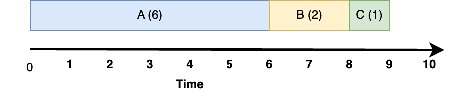
Fig. 10.2 FIFO with tasks run in order A, then B, then C

So the average turnaround time is: \((6 + 8 + 9)/3 = 7.7 min\)

On the other hand, if the tasks are run in the order C, B, A, they will execute on the processor as shown below.

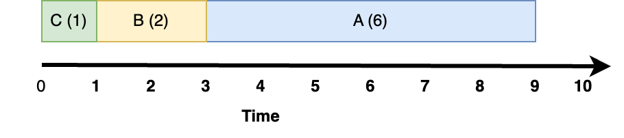
Fig. 10.3 FIFO with tasks run in order C, then B, then A

So the average turnaround time is: \((1 + 3 + 9)/3 = 4.7 min\)

We see here that when short tasks are processed after long tasks the long ones have a major impact on the short ones, while if the order is reversed, the impact on the long tasks running after the short ones is much less.

10.2.1.1. Tradeoffs

• Requirements:

  • requires no information from user

• The Good:

  • a very simple algorithm; can make sense for Batch since there is no context switching

• The Bad:

  • Poor average turnaround time

  • Not appropriate for response time sensitive since they don’t get to run until all tasks ahead of them have completed and no mechanism to support real time workloads

  • Doesn’t do anything to maintain high utilization of non-CPU resources

10.2.2. Shortest Job First (SJF)

For some systems, for example Batch, we know a-priori how long a task will take. Hence, rather than running them in the order they arrived, we can sort them based on how long the tasks will take and always run the shortest tasks first to get the better turnaround time shown in Fig. 10.3. This policy is called shortest job first, and will always yield the optimal turnaround time.

Let us, however, consider the case below, where tasks A and B arrive at time 0, and tasks C, D, and E arrive at time 3.

Task	Start	Runtime (min)
A	0	2
B	0	4
C	3	1
D	3	1
E	3	1

If we run jobs to completion we will get the following:

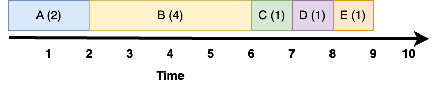
Fig. 10.4 SJF without preemption

So the average turnaround time is: \((2+6+(7-3)+(8-3)+(9-3))/5 = 4.6 min\)

If we instead preempt B to run the new jobs who’s time is shorter than B’s remaining time, we get the following execution:

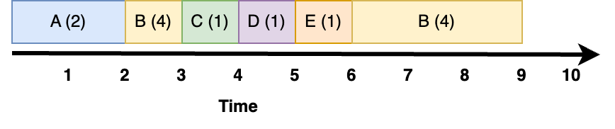
Fig. 10.5 SJF with preemption

With a shorter average turnaround time of \((2+(4-3)+(5-3)+(6-3)+9)/5 = 3.4\)

This demonstrates the value of preemption, where we can stop long running tasks to get short ones in and out of the system quickly.

To understand the major problem with Shortest Job consider what happens if one minute tasks continue to arrive every minute starting at minute 4. B will never complete, or in scheduling terminology, it will starve even though the system is processing work as fast as it is arriving. Starvation is a major problem with a pure shortest job first algorithm.

10.2.2.1. Tradeoffs

• Requirements:

  • requires knowledge of task run time

• The Good:

  • Optimizes turn around time

  • Great for Batch

• The Bad:

  • Not appropriate for response time sensitive that perform I/O

  • Can result in starvation

  • Doesn’t do anything to maintain high utilization of non-CPU resources

10.2.3. Round Robin

With SJF, we found that if we preempt a long running task when a short one arrives, we can improve turn around time. In many environments, we don’t know how long a task will take, and, rather than just using the CPU, many tasks switch back and forth between using the CPU and doing I/O.

We illustrated in Fig. 10.1 how a CPU and I/O intensive application might use the CPU. For such tasks, if we can make sure that CPU intensive tasks don’t block I/O intensive ones for too long, the system will enable the I/O intensive ones to better use the I/O devices while the CPU intensive task has only modest impact from the short periods of time that the I/O intensive ones use it. Also, if a user is interacting with the I/O intensive one, e.g. running emacs, the Response Time is less affected by the CPU intensive applications.

The Round Robin algorithm builds a simple FIFO run queue of tasks in the ready state much like the FIFO algorithm described earlier. When a task starts running it is given a fixed amount of time to run, often called a Quantum or Time slice. When the quantum expires the OS does a context switch to the next task in the queue and adds the previously running task at the back of the queue.

Let us consider a situation with three tasks shown in the table below:

Task	Start	Runtime
A	0	6
B	0.0001	2
C	0.0002	1

Assuming the units are in seconds, let us assume that the quantum is also (unrealistically) 1 second. In that case, a round robin scheduler will run tasks as shown in Fig. 10.6 below:

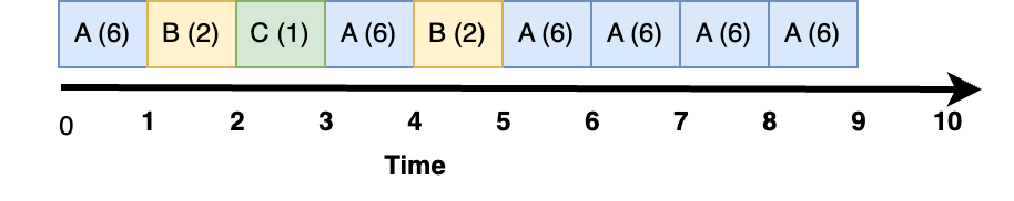
Fig. 10.6 Round Robin scheduling, where every task executes for a quantum of time.

The average turnaround time of this round robin schedule is \((3 + 5 + 9)/3 = 5.6\). We can see that it is terrible compared to SJF, but much better than the worst FIFO case.

The preemptive scheduling models introduces a new parameter we need to set: the length of the quantum. We have to weigh the cost of changing processes against the interactivity requirements when deciding on the length of a time we will run CPU intensive tasks. You want to pick a time large enough that you are amortizing the cost of a context switch; if you picked a time that was a few hundred computer cycles you would be spending most of your time context switching. On the other hand, if you it is too long, interactive tasks would get terrible response rate.

Let us assume that the quantum is, say 10msec, a number much larger than the time for a context switch but reasonable to not add much delay to tasks that interact with humans. Also, we will assume that we can ignore the context switching time. We can represent what happens is shown below:

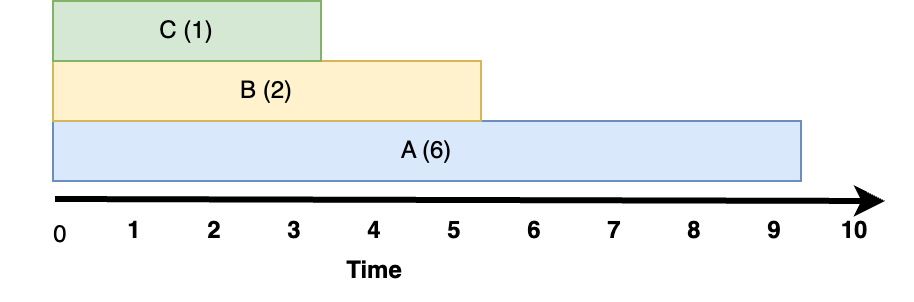
Fig. 10.7 Round Robin scheduling, with a reasonable quantum.

For the first three seconds, all three tasks share the CPU. Assuming that each gets an equal share, C will have had a full second of compute time after three seconds and it will be done. From seconds 3-5 the CPU is shared by tasks A and B, where each get half of it. After 5 seconds, B will have had two full seconds of compute time, and A will have the CPU to itself from that point forward.

10.2.3.1. Tradeoffs

• Requirements:

  • requires no knowledge of task run time

• The Good:

  • Simplest preemptive algorithm, better for response time than any non-preemptive one

  • Does better for non-CPU resource use than any non-preemptive algorithm

• The Bad:

  • Can still result in poor response time with many CPU intensive tasks

  • Poor turnaround time

  • Bad for batch since constant context switching, and real time since difficult to make any prediction on how long tasks will take